

Our goal with Klang Pianissimo was to make accurate Swedish transcription fast enough to process large amounts of audio. We started from NVIDIA's Parakeet v3, a 0.6B-parameter FastConformer-TDT model. It is a very fast model that is already trained on a large set of languages. However, as we show in the benchmarks below, its word error rate (WER) on Swedish is 17% compared to 7% for Whisper large v3 and 3.5% for KB-Whisper large. We decided to see how far we could push the performance by specializing it on our dataset of Swedish audio and transcripts.
Building the training data
We started with a collection of over 90,000 hours of Swedish speech from publicly available material, including parliamentary data from RixVox, subtitles and open datasets. The material varied in recording quality, speaking style and how closely the accompanying text followed the speech.
We had to filter away a lot of data that was not good enough to train on. Firstly, we did language identification on both the audio and the text, removed duplicate material, and rejected references with excessive repetition, implausible text density or corrupted text. We used text processing to repair malformed Unicode and removed nonspoken formatting.
We also used voice activity detection (VAD) to filter based on how much of each recording contained speech, and we checked whether the text covered a reasonable share of its duration.
This removed a lot of clearly bad references; however, the most powerful filter was forced alignment of the text to the audio. By using a different model to locate each word in the audio, we could find clips where the audio differed substantially from the reference. It also caught references with inaccurate timestamps and let us add timestamps where none existed.
These checks removed many obvious problems. However, one problem remained: missing text. The alignment method scored how well each word matched the audio, but did not tell us whether any text was missing. A reference could still be fluent Swedish and leave out large parts of what was said.
Transcripts, and in particular subtitles, often shorten passages, remove repetitions or omit whole exchanges. Too many omissions in the reference texts will teach the model to omit speech too. Whereas Whisper uses a Transformer decoder that attends across the encoded audio, Parakeet uses a much smaller decoder. It consists of a two-layer LSTM and a small joint network that combines the LSTM's output with the current encoder frame. This makes it much harder for the model to learn to rewrite sentences or skip words based on context.
We therefore measured reference coverage separately. We detected speech activity in the recording and compared it with the intervals covered by aligned words. A sustained stretch of speech without corresponding text gave us a signal that the reference was incomplete.
This check was applied when generating training examples from the source data. This let us retain useful passages without having to accept or discard an entire recording.

In total, all filtering removed roughly 45% of the estimated 90,000-hour collection, leaving over 50,000 hours in the broad training set.
Training on a changing mixture
We used curriculum learning, shifting the training data towards cleaner references as training progressed. The aim was to learn from the variety in a large collection first, then refine the model's transcription on a smaller set of more reliable examples.
We selected clips with strong alignment and better reference coverage for the strict subset. This left about 4,000 hours of high-quality data.
We used the bulk collection for roughly 86% of the training iterations. We then spent about 4% of the total iterations on a mixed phase, sampling roughly half the clips from the bulk collection and half from the strict subset. Lastly, we finished with 10% of the iterations on the high-quality dataset.

Augmentation
We also added augmentation to the training data. This allows us to artificially extend the size of the dataset by training the model on multiple variations of the same audio. These variations exposed the model to recording conditions that were less common in the original data. We used the following types of augmentation.
Reverberation and background noise. We used real and simulated room impulse responses to reproduce the reflections a microphone picks up in a room. We convolved the speech with a room response, restored its overall level, then mixed in noise at signal-to-noise ratios between 5 and 20 dB. For this augmentation, we used recorded and simulated room impulse responses as well as background noise from MUSAN's noise collection.
Audio compression. To reproduce the artifacts of heavily compressed audio, we encoded and decoded clips with Opus at bitrates from 6 to 24 kbit/s.
Restricted bandwidth. We removed high-frequency detail with a low-pass filter, sampling the cutoff between 3.4 and 7.8 kHz.
In the broad collection, 15% of clips received reverberation and noise, 20% compression and 10% bandwidth restriction. Each clip received at most one of these transformations, leaving 55% with their original audio. We processed and saved these variations before training so the more expensive augmentation would not slow down training. For the strict subset, we saved the original audio.
During training itself, we varied gain and clip boundaries for both selections. We changed gain by up to 6 dB in either direction and added short stretches of synthetic room tone at the edges, so speech would not always start and end at the clip boundaries. Each end independently had a 20% chance of receiving 0.1-1.5 seconds of padding. We based the padding level on the quietest short interval in the clip, giving it a noise floor suited to the recording.
Gain and padding were sampled again each time a clip was used. This kept some variation in the input even in the final stages, where we trained repeatedly on a smaller set of examples.
Batch normalization
The batch normalization (BatchNorm) layers in Parakeet's encoder behave differently during training and inference. During standard training, they normalize activations in the convolution blocks using the current batch's mean and variance. They separately maintain exponential moving averages of those statistics, which are saved in the checkpoint. At inference, these saved estimates are used for normalization.
Batches with certain characteristics appeared so rarely that they were poorly represented in the moving averages. The model performed well on these batches during training, because they were normalized using their own statistics, but poorly at inference, when the saved estimates were used instead.
We therefore normalized activations using a weighted average of the current batch's statistics and the moving averages. Early in training, we relied almost entirely on the current batch to keep training stable. We gradually shifted the balance towards the moving averages, bringing normalization closer to inference behaviour as training progressed.
At that point, we benchmarked the model on multiple test sets and thought it was ready to be released.
A problem with long recordings
When we finally tested the model on long recordings, the error rates were unexpectedly high compared with the short-clip benchmarks. The model dropped words, sentences and sometimes whole passages.
To process long recordings efficiently, we use local attention with 256 encoder frames on either side, about 20.5 seconds in each direction at each layer. This keeps attention cost linear in recording length. However, a different part of the model still depended on the entire recording: the input normalization.
Before audio reaches the encoder, the preprocessor converts it into 128-band log-mel features and normalizes each band using its mean and standard deviation over the input. In training, those statistics came from clips usually lasting 10 to 30 seconds. When transcribing a long recording, they could come from hours of audio containing different speakers, background conditions and stretches of silence.
The same passage could therefore reach the encoder with vastly different values, depending on audio in other parts of the recording. With local attention, the model cannot account for audio outside its attention window. Our short training clips had not exposed the model to this mismatch.
Testing the explanation
To test whether normalization explained the missing speech, we normalized each input mel frame using the mean and standard deviation of each frequency band over a 40-second window centred on that frame. The window moved with each frame, keeping the normalization local throughout the recording. We kept the weights and local-attention settings fixed and transcribed the recording in one continuous pass. WER fell from 11.1% to 5.1%, without retraining.
The sliding window solved the problem, but we wanted to find a solution that didn't involve changing the preprocessor.
A small final fine-tune
We therefore tried to teach the model to handle the difference instead. We kept training on short clips, but adjusted their features to mimic what the model would see when those clips were part of a much longer recording.
We measured the differences between short-window and whole-recording normalization on about 38 hours of audio from 22 recordings. This gave us over 3,000 real patterns describing how frequency bands changed together.
We used these patterns as a new augmentation on the clips already in our training set. Half the clips received a sampled pattern at varying strengths. Using patterns from real recordings preserved the relationships between frequency bands, so the augmented features resembled the changes we had seen in long-form inference.
We continued training on the existing strict mixture, and the problem was resolved after just 0.3% of a full training run.
Recovering the missing speech
After the fine-tune, WER on the long-form clip fell from 11.1% to 4.7% using the original whole-recording normalization. In particular, deletions dropped from 8.4% to 2.2% of reference words, accounting for most of the improvement.
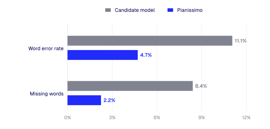
Whole-recording and moving-window normalization now both gave 4.7% WER on the file. The improvement also extended to the other long recordings we tested, while short-clip scores remained unchanged.
Evaluation
We compared the final model Pianissimo with 13 other open models, both in terms of Swedish recognition quality and transcription speed.
Swedish recognition
The table covers results on the Common Voice Swedish v26 test and development sets, Swedish FLEURS, Klang Dialects and an internal read-speech set. The mean gives equal weight to each of these five datasets.
Scroll to see all datasets →
| Model | Mean | Common Voice test | Common Voice dev | FLEURS | Klang Dialects | Internal read speech |
|---|---|---|---|---|---|---|
| Pianissimo | 4.5% | 4.5% | 4.5% | 6.5% | 4.9% | 2.0% |
| Parakeet v3 | 17.7% | 18.5% | 17.5% | 15.2% | 25.8% | 11.5% |
| KB-Whisper large | 3.5% | 3.9% | 4.0% | 5.1% | 2.3% | 2.3% |
| KB-Whisper medium | 4.9% | 5.4% | 5.3% | 6.6% | 3.6% | 3.5% |
| KB-Whisper small | 5.8% | 6.3% | 5.9% | 7.7% | 5.2% | 3.7% |
| Whisper large-v3 | 7.2% | 8.1% | 8.1% | 7.2% | 8.2% | 4.5% |
| KB-Whisper base | 7.6% | 8.4% | 8.3% | 9.6% | 7.7% | 3.8% |
| Whisper turbo | 10.4% | 13.2% | 12.2% | 8.5% | 13.7% | 4.6% |
| KB-Whisper tiny | 10.9% | 12.3% | 11.8% | 13.1% | 12.6% | 4.8% |
| Canary 1B v2 | 12.2% | 14.5% | 14.6% | 9.6% | 15.6% | 6.6% |
| Qwen3-ASR 1.7B | 20.8% | 22.1% | 21.7% | 19.6% | 26.2% | 14.2% |
| Nemotron 3.5 ASR 0.6B | 27.8% | 30.4% | 32.4% | 24.4% | 35.4% | 16.3% |
| Qwen3-ASR 0.6B | 36.7% | 38.0% | 38.0% | 35.9% | 44.5% | 27.0% |
| VibeVoice-ASR 8B | 100.1% | 123.9% | 121.8% | 81.1% | 130.1% | 43.6% |
Compared with Parakeet v3, Pianissimo reduces WER by 76% on Common Voice test, 57% on FLEURS and 81% on Klang Dialects. KB-Whisper large remains more accurate on those datasets, but Pianissimo gets close to its recognition quality at much higher throughput.
Before scoring, we lowercased text, replaced punctuation with spaces and collapsed whitespace. We did not do any normalization of numbers. Note that VibeVoice relies on automatic language identification and frequently returned text in another language on these short clips.
Transcription speed
Parakeet's speed was one of the main reasons we chose it. We compared Pianissimo's speed with that of the other open models above. We used batches of 30-second clips to compare how much audio each model could process in bulk. We chose this clip length to favour the Whisper models, which pad shorter clips to 30 seconds.
The benchmarks were conducted on a single NVIDIA A100 card. We ran each model in its default framework, tested different batch sizes and precision settings and picked the fastest recorded configuration for each model. We warmed the models before timing, synchronized GPU work and reported median processing times, excluding model loading. More details are found under "Benchmark settings" below.
Pianissimo processed about 41 hours of audio in one minute, approximately 2,500× realtime. In the same benchmark, KB-Whisper medium reached 66× realtime and KB-Whisper large 39×.
The graph combines this throughput with the mean WER from the table above, showing how far Pianissimo has shifted the trade-off between speed and recognition quality.
Benchmark settings
Precision and batch sizes below refer to the throughput runs.
- Pianissimo, Parakeet v3 and Canary 1B v2: NVIDIA NeMo, bfloat16, batch 128. Canary was set to Swedish.
- KB-Whisper and Whisper: Hugging Face Transformers, float16, Swedish, 30-second chunks. Batch sizes: KB-Whisper tiny 128; base, small and medium 64; KB-Whisper large and Whisper large-v3 32; Whisper turbo 8.
- Nemotron 3.5 ASR 0.6B: Transformers, bfloat16, batch 32, Swedish, 13 lookahead tokens (1.12-second chunk latency).
- Qwen3-ASR 0.6B and 1.7B: Transformers, bfloat16, batch 32. Swedish was specified for transcription, with a 440-token output limit.
- VibeVoice-ASR 8B: Transformers, bfloat16, batch 32, 440-token output limit. Only the transcript text was scored.
To push throughput even further, we transcribed a single long recording in batches on an H100 GPU. With that setup, it's possible to reach over 4,000× realtime, equivalent to over an hour of audio per second of model processing!
Using Pianissimo
You can download the weights at KlangAI/pianissimo-sv on Hugging Face, under CC BY 4.0. The repository includes loading instructions so you can run the model on your own recordings and infrastructure.
For the release overview and why we are making the model available openly, see Introducing Klang Pianissimo.