Unlikely similar voices - Klang Research

In the first part of this article we described how voices are turned into speaker embeddings, how much a single voice varies between meetings, and how we warped the embedding space to make different voices easier to tell apart. We ended with two questions: How often is it ok to misidentify a voice? And is there more we can do to make that even more unlikely?

Averaging away the noise

A single clip is often not good enough for identifying someone. Several things like distance to the microphone, mumbling and background noise negatively affect the accuracy. So instead of comparing single clips, we average the embeddings of several clips from the same meeting, in the hopes of reducing this effect. This turned out to significantly reduce the rate at which we misidentify people (measured by equal error rate), from 3% to 1% when averaging just three short clips.

We also tried to embed longer clips to reduce the variance, but this was far from as effective. Measuring at different times in a meeting is much more efficient at capturing different conditions, and therefore results in more reliable embeddings.

The same trick works across meetings. Once a speaker has been identified in several meetings, we combine clips from all of them into a single embedding for that person. A voiceprint built from several meetings matches new recordings noticeably better than one built from a single meeting, because it also averages away the conditions of any particular day. This also means that identification in Klang improves with use, every confirmed name makes the voiceprint a little better.

Voices we have never heard

The analysis so far has been based on the assumption that we are trying to match a voice to a set of known speakers. However, this is often not the case. Meetings are full of guests, customers and new colleagues. The question we have to answer is therefore not "Who does this voice belong to?", but "Does this voice belong to anyone we know, and if so, who?". The difference might seem small, but it changes the problem from finding the most similar voice, to deciding if two voices are similar enough.

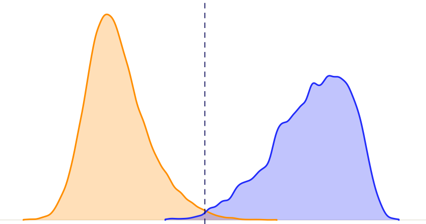
We therefore need to set a cutoff for when two voices count as one person. If the best match scores above the cutoff, the voice gets that name. Below it, the voice stays unknown. Choosing the cutoff is a tradeoff between two mistakes:

If it is too low: then strangers get matched to somebody they happen to sound like
If it is too high: then we fail to recognize people we should know.

Two overlapping similarity distributions: different people centered near 0.1, the same person across meetings centered near 0.7, with a dashed cutoff line between them — Similarity between recordings of the same person and between different people, measured on our internal meetings with three-clip averages in the corrected space. The dashed line is the cutoff where 1% of strangers score above it. Anything orange to its right would get a wrong name, anything blue to its left goes unrecognized.

If we allow 5% of strangers to be wrongly matched, then we can recognize about 99% of returning voices. That might sound good, but it is the wrong balance for Klang. A wrong name in a transcript will spread into summaries, search results and analysis. On the other hand, choosing "unknown" can always be quickly corrected by the user. We would therefore much rather leave a voice unnamed than guess. That means using a far stricter cutoff, but measuring what happens at strict cutoffs turned out to be trickier than expected.

Measuring rare mistakes

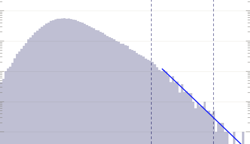
Our internal dataset contains at most a few hundred different people. We can use this as our set of strangers, but if we want a cutoff where only 1% are misidentified, that cutoff is determined by the two highest scoring strangers. That is by far too few examples to give any sort of confidence, so we needed far more strangers than our own meetings could provide.

This is where the public dataset from the first part became important again. It contains over 400,000 clips, which might sound like more than enough. But many of the clips come from the same person, a member of parliament can give hundreds of speeches. Counted properly, those 400,000 clips contain closer to 8,000 distinct voices. And at 8,000 strangers, the 1% cutoff is determined by 80 people instead of two, a much more reliable measure. However, the other part of the question is then how good our recall is, i.e. how well we actually recognize a person in a new setting, now that we have such a high cutoff. Since we have over 500 different speakers from our parliamentary data, each having multiple recordings on different days or even years, we can actually get a good estimate of recall too.

But we wanted to go further than 1%, we wanted it to be extremely unlikely that we mislabel a speaker. But at a cutoff where only 0.01% of strangers are misidentified, even 8,000 voices are not enough, and we are back to relying on a few extreme outliers. To solve this, we applied tools that have been developed for a completely different case of extreme outliers: flood statistics. Instead of trying to measure how often a 400-year flood occurs, you fit a curve to the largest floods on record and extend it. The highest scoring strangers behave the same way, so we can fit a curve to the whole set of outliers. We can then get accurate estimates of the cutoffs based on this curve, instead of from a few lucky data points.

Histogram of similarity scores for 100,000+ pairs of different parliament speakers on a logarithmic axis, with a fitted curve extending through the sparse extreme tail — Similarity for every pair of the 500+ parliament speakers: 100,000+ pairs of genuinely different voices. The dashed lines mark the top 1% and top 0.01% of scores. Out in the far tail, single pairs are all the data there is (the right-hand scale counts individual pairs), so the strictest cutoffs are read from the flood-style fit instead.

Being careful turned out to be cheap

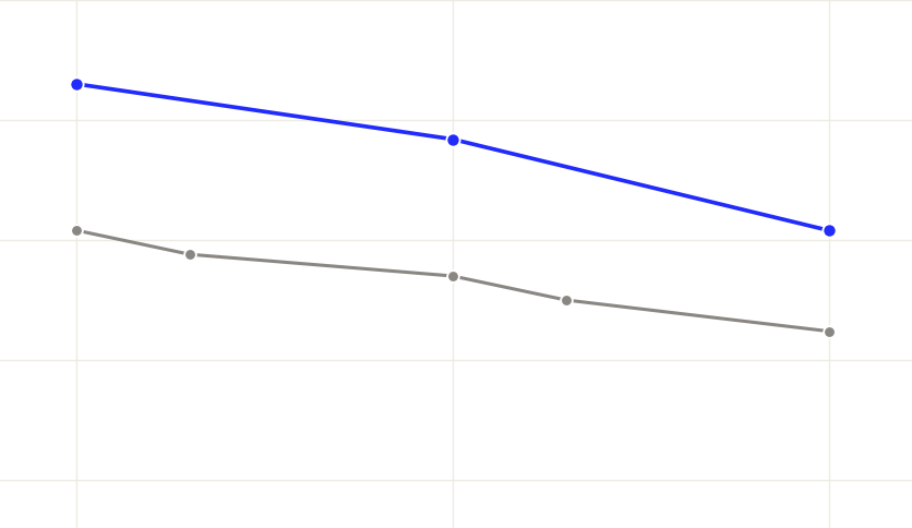
With the combination of 8,000 voices and the flood-style curve, we could finally measure cutoffs all the way down to 0.01%, i.e. where only one stranger in 10,000 would be misidentified. The result was surprisingly good. Making the cutoff a hundred times stricter, from 1% down to 0.01%, only lowered the recognition rate by a few percentage points. And by combining this with the warping we mentioned earlier, we were able to achieve over 90% recall at the 0.01% cutoff.

Recognition rate versus strictness of the cutoff on a logarithmic axis, staying between 86 and 96 percent as the cutoff tightens a hundredfold — Share of returning voices we recognize as the cutoff tightens from 1% of strangers wrongly matched down to 0.01%, measured on the public dataset.

This is how we modeled voice recognition in Klang. A name is only applied automatically when the similarity is clearly above the strict cutoff. If the model is unsure, then we display a suggestion that can be confirmed with a simple click instead. And every confirmation nudges the voiceprint to make it even more accurate in the future.